How to perform a genomic control computation

Figure 1 displays the QQ plot generated from the P-values obtained by performing GLM-GWAS calculations with demo data. As you can see, the points on the plot significantly deviate from the red diagonal line, moving sharply upwards and to the right with a very large slope. This phenomenon is referred to as genomic inflation.

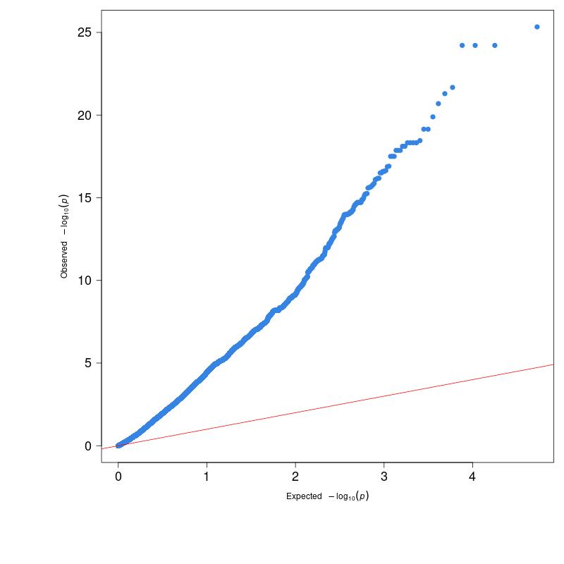
(Figure 1)

Figure 2 shows the Genomic Control tab after completing the genomic control calculation. This was done by selecting the “pvalues” file (a result file generated after either GLM-GWAS or LMM-GWAS analysis) and clicking the [Execute] button. The file generated from the genomic control calculation is saved in the same folder as the input file (pvalues).

Here’s an explanation of the files created by the genomic control calculation:

1. gc_pvalues: This file contains the P-values that have been adjusted through the genomic control calculation.
2. lambda: This value (ranging from 0-1) indicates the strength of genomic inflation. A lambda value closer to 1 means the genomic inflation is stronger. Conversely, a value closer to 0 indicates that the P-values better follow a chi-squared distribution with 1 degree of freedom.

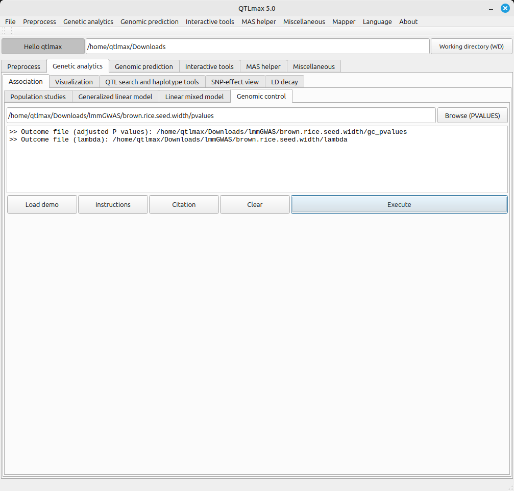
(Figure 2)

Figure 3 shows the project folder after the genomic inflation calculation. You can see that the gc_pvalues file and the lambda file are now present alongside the existing GWAS result files.

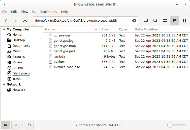
(Figure 3)

Figure 4 shows the newly drawn QQ plot using the adjusted P-values contained in the “gc_pvalues” file. As you can see, the P-values now follow the red diagonal line relatively well.

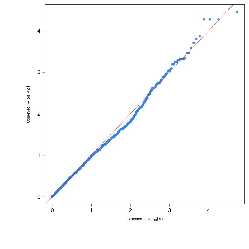
(Figure 4)

Figure 5 shows the lambda value (lambda GC = 6.515145) calculated during the genomic inflation process.

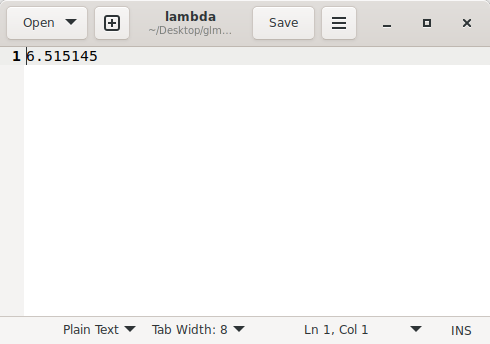
(Figure 5)