PCA computation

Figure 1 shows the PCA tab page selected.

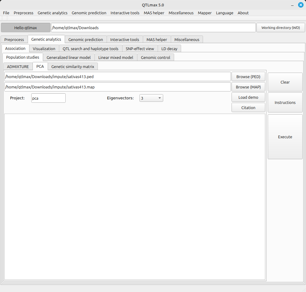
(Figure 1)

Figure 2 shows the project folder containing the result files after the PCA calculation is complete.

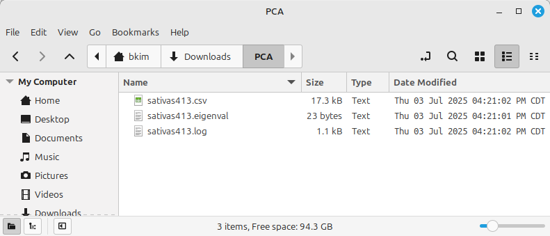
(Figure 2)

Figure 3 shows the contents of the PCA result file (.CSV). Each column labeled as PC1, PC2, PC3, etc., is referred to as a Principal Component.

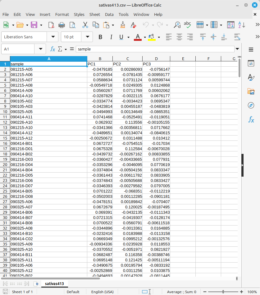
(Figure 3)

Figure 4 shows the contents of the file (*.eigenval) that displays the eigenvalue corresponding to the Principal Components (PC1, PC2, etc.).

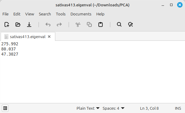
(Figure 4)

QTLmax Workbench allows you to generate PCA plots. To draw a PCA plot, a PCA result file in CSV format is required. Before importing the PCA result file, you must add a new column to the far right and enter information about the group each individual belongs to (Figure 5). This step is necessary to visualize the distribution of each group by color on the PCA plot.

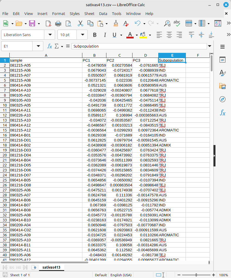
(Figure 5)

Figure 6 shows the PCA plot tab page selected in QTLmax Workbench. This tab page has many setting options. If you don’t want to select each setting option individually, just click the [Load demo] button. You’ll see most of the setting options are configured automatically.

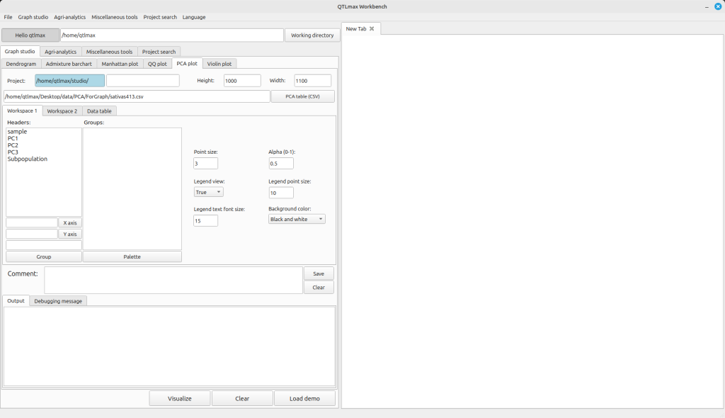
(Figure 6)

After replacing the demo data with your own, you are free to change the settings to your desired values. You also must assign colors to each group. To do this, select a group and click the [Palette] button. A palette window will appear, where you can choose the desired color for each group. Once all settings are complete, click the [Visualize] button. Finally, you’ll see the PCA plot drawn (Figure 7).

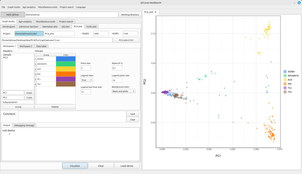
(Figure 7)