Genetic similarity matrix computation

Figure 1 shows the tab page selected for calculating the “genetic similarity matrix.”

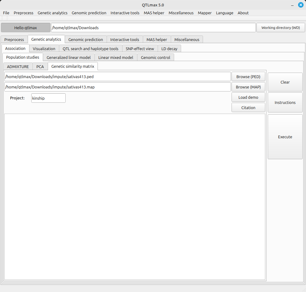
(Figure 1)

Figure 2 shows the result files listed in the project folder. The file with the CSV extension contains the calculated genetic similarity matrix results.

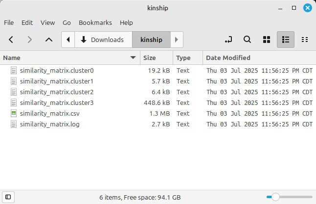
(Figure 2)

Figure 3 shows the resulting genetic similarity matrix. You can see that all diagonal values of the matrix are 1, and all other values are between 0 and 1.

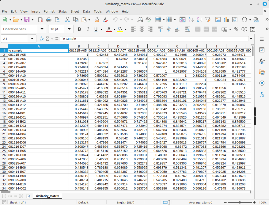
(Figure 3)

You can draw dendrograms from the calculated genetic similarity matrix using QTLmax Workbench; by using it, you can draw the following two types of dendrograms:

1. Circular dendrogram
2. Plain dendrogram

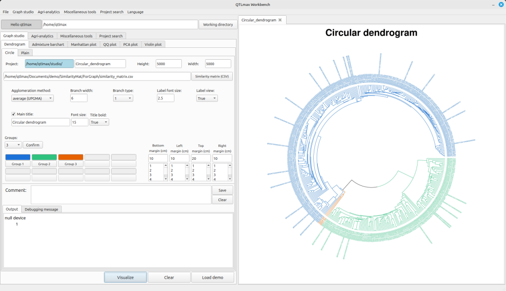
Figure 4 shows the tab page in QTLmax Workbench that supports dendrogram plotting. If you find it tedious to manually specify each option, click [Load demo]. You’ll then see all the settings automatically filled in (Figure 4).

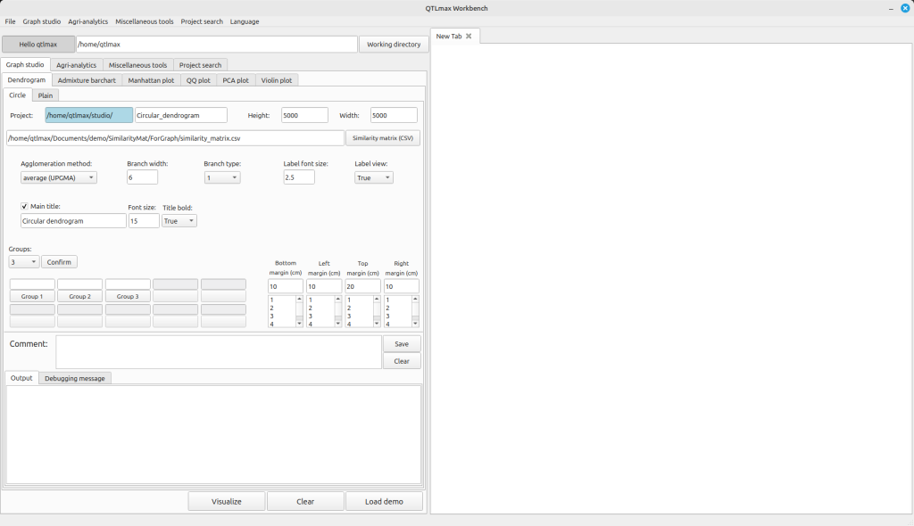
(Figure 4)

After clicking the [Similarity matrix (CSV)] button, you can replace the demo data with your own, followed by changing the settings to your desired values. You can select a number from the combobox on the left side of the [Confirm] button. This number represents how many groups you want to divide the entire population into. Once you select a number, you will see that many buttons below it become active, each labeled (e.g., [Group 1], [Group 2], [Group 3]). Clicking each button will display a pop-up palette where you can choose a color for that specific group. After finalizing all your settings, click the [Visualize] button to draw the dendrogram. Figure 5 shows a dendrogram drawn after dividing the entire population into two groups.

(Figure 5)