This post explains how to perform the LMM-based GWAS procedure. This feature is powered by the computational engine of GWASpro; you can find the original research paper here: https://academic.oup.com/bioinformatics/article/35/14/2512/5227981.
This feature requires the following input files:
- A set of imputed PED and MAP files
- A kinship matrix (e.g. Genetic similarity matrix, VanRaden K matrix, Pedigree Kinship matrix, Genomic Kinship matrix)
- A preprocessed phenotype file that has been merged with either a PCA or an Admixture table. In order to learn about how to merge phenotypic dataset and a multivariate table about population structure, you can visit here: https://open.qtlmax.com/guide/index.php/2025/07/03/merging-phenotype-and-pca-tables/
It is important to note that all input datasets mentioned above can be generated within QTLmax 6.0, allowing them to be seamlessly integrated into this feature for the GWAS procedure. For the kinship matrix and preprocessed phenotypic files, you can choose the most appropriate options for your specific analysis.
Figure 1 shows the ‘GWAS’ tab with all input datasets loaded. Once you have uploaded a preprocessed phenotypic dataset, the column headers from the file will be automatically populated in the central panel, as shown in Figure 1.
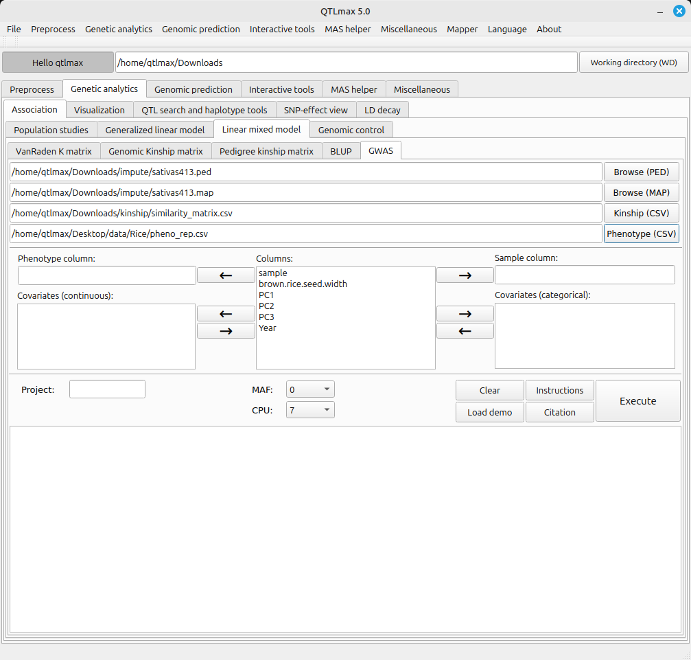
(Figure 1)
The LMM-GWAS tab requires a few settings. Here’s how to configure each one:
- Send the header value that specifies the sample to the “Sample column” text box.
- Send the header value that specifies the phenotype value to the “Phenotype column” text box.
- Send the header values that specify the PCA values (e.g., PC1, PC2, PC3) to the “Covariate (continuous)” panel.
- If there are any categorical header values that specify environmental factors (e.g., location, year, replication, treatments), send them to the “Covariates (categorical)” panel.
In case you handle numerous SNPs and samples for GWAS, its computational cost will be hefty; it essentially constitutes massively numerous independent computations. This challenge can be technically tackled by parallel computing. QTLmax 6.0 supports parallel computing in a manner of divide-and-conquer, which can be used simply by selecting the number of CPU threads from the dropdown menu labeled ‘CPU’.
With all settings configured, pressing the [Execute] button will kick off the GWAS process. During the process, a pop-up terminal will appear, displaying a progress bar moving forward. Figure 2 shows the interface after the GWAS has finished.
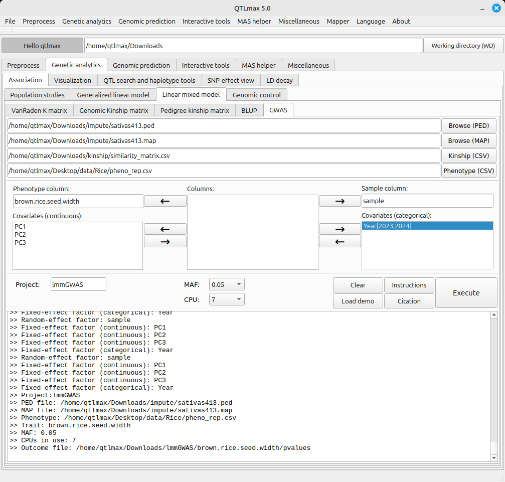
(Figure 2)
The path to the LMM-GWAS calculation result files is as follows:
[Working directory] > [Project folder] > [trait folder]
Figure 3 shows the resulting files created as a result of the GWAS. Key output files are as follows:
- genotype.ped, genotype.map: A set of SNP files used for the GWAS computation. These have been trimmed and sorted to ensure that all input files are perfectly aligned based on their entry (sample) names.
- pvalues: A list of the resulting P values from the GWAS computation. Essentially, its records are perfectly aligned with the ‘genotype.map’.
- gwas_settings.proj: A project file that stores the configuration used for the analysis.
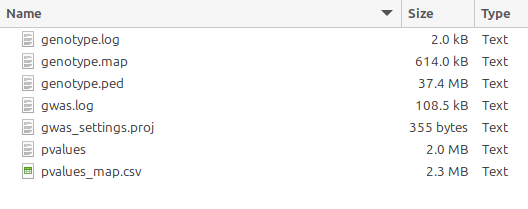
(Figure 3)
The output files can be used for further analysis, such as genomic control, Marker-Assisted Selection (MAS), and haplotype investigation, etc. If you want to look into the GWAS output in a human-readable format, the ‘pvalues_map.csv’ file is the appropriate choice. (Figure 4)
***** It is important to note that the P values are calculated using the Wald test. *****
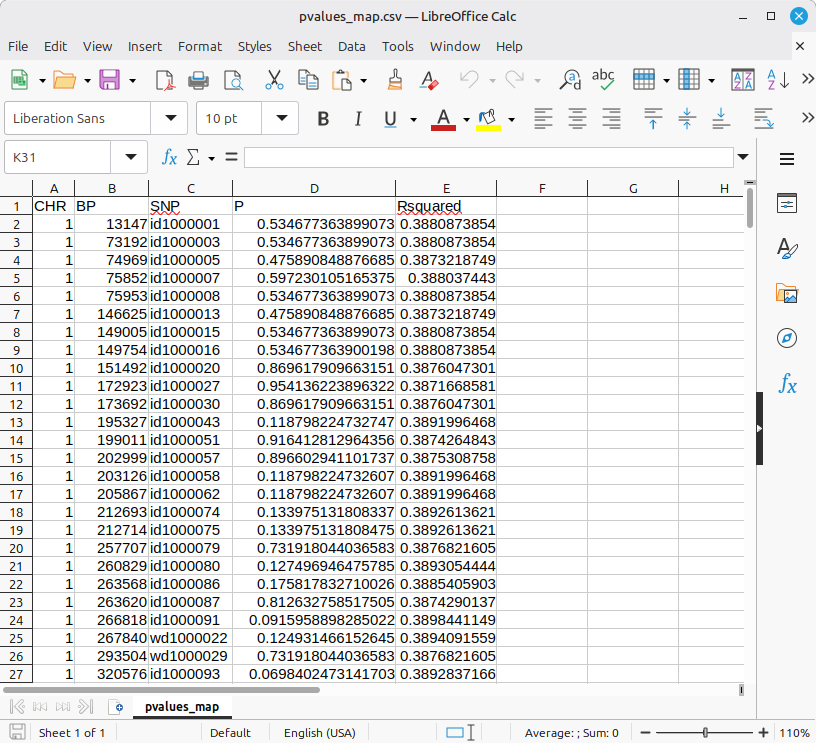
(Figure 4)